Rkeyline is an R package to support desktop keyline design planning and terrain analysis from Digital Elevation Models (DTMs). It provides a complete workflow from raw DTM data to approximate keyline design, covering geomorphological analysis, valley and ridge network extraction, and visualization.
Note: Generated keylines are computational approximations for desktop planning only. Always verify and adjust keylines on-site with an experienced practitioner before implementation.
Installation
# install.packages("remotes")
remotes::install_github("Lenaelu/Rkeyline")
Dependencies
Make sure you have the following packages installed:
install.packages(c("terra", "sf", "dplyr", "smoothr", "shiny", "viridis"))Rkeyline also requires WhiteboxTools, which is used for hydrological processing (depression filling, flow direction, flow accumulation, and stream extraction) and for converting raster stream networks to vector lines. WhiteboxTools cannot work with R objects directly — it reads and writes files on disk, which is why a persistent output folder is required.
install.packages("whitebox")
whitebox::install_whitebox()
Important: Output Folder
Several functions use WhiteboxTools under the hood, which requires intermediate files to be written to disk. You must specify an output_folder that exists and is writable on your system. Both calc_geomorph_metrics() and extract_networks() need access to the same folder — files written in Step 2 are read again in Step 3.
Note:: Do not rely on the default
tempdir(). Temporary directories are cleared when your R session ends, so if you restart R between steps the intermediate files will be gone andextract_networks()will fail. Always set a persistent folder explicitly.
# Set once and reuse throughout the entire workflow
output_folder <- "C:/my_project/rkeyline_temp"   # Windows
output_folder <- "/home/user/my_project/temp"     # Mac/Linux
The following files are written by calc_geomorph_metrics() and must still be present when extract_networks() runs:
-
temp_dtm.tif,dtm_filled.tif,flow_pointer.tif,flow_acc.tif,streams.tif -
dtm_inverted.tif,dtm_filled_inverted.tif,flow_pointer_inverted.tif,flow_acc_inverted.tif,streams_inverted.tif
Temporary shapefiles created by extract_networks() are deleted automatically after use.
Workflow Overview
The package follows a clear step-by-step workflow:
DTM → calc_geomorph_metrics()
         ↓
      extract_networks()        (valleys & ridges)
         ↓
      extract_main_valleys()
      extract_main_ridges()
         ↓
      create_keylines()
         ↓
      plot_*() functions
Usage
A small example DTM is included in the package to get started quickly. You can use it to run the full workflow without needing your own data:
library(terra)
library(Rkeyline)

# Load the built-in example DTM
dtm <- terra::rast(system.file("extdata", "example_dtm.tif", package = "Rkeyline"))
Or load your own DTM:
dtm <- terra::rast("path/to/your/dtm.tif")Step 1: Set your output folder
# Define your output folder once and reuse throughout the workflow
output_folder <- "C:/my_project/rkeyline_temp"   # Windows
output_folder <- "/home/user/my_project/temp"     # Mac/Linux
Step 2: Calculate geomorphology metrics
This is the foundation of the entire workflow. Run it once and reuse the results. WhiteboxTools writes intermediate raster files to output_folder — these must remain available for Step 3.
metrics <- calc_geomorph_metrics(dtm, output_folder = output_folder)Returns slope, aspect, hillshade, contours, flow accumulation, stream networks, and their inverted equivalents for ridge analysis.
Key parameters:
-
output_folder— path for WhiteboxTools intermediate files (must be the same in Step 3) -
contour_interval— elevation spacing for contours (default: 10) -
stream_threshold— number of cells required to form a stream (default: 1000) -
breach_dist— maximum breach distance for depression filling (default: 50)
Step 3: Extract valley and ridge networks
WhiteboxTools reads the intermediate files written in Step 2. Pass the same output_folder as in Step 2.
valleys <- extract_networks(dtm, type = "valley", metrics = metrics, output_folder = output_folder)
ridges  <- extract_networks(dtm, type = "ridge",  metrics = metrics, output_folder = output_folder)
Step 4: Extract main valleys and ridges
Select the top N valley and ridge lines ranked by flow accumulation.
main_valleys <- extract_main_valleys(valleys, dtm, nr_main = 2, metrics = metrics)
main_ridges  <- extract_main_ridges(ridges,  dtm, nr_main = 2, metrics = metrics)
Step 5: Generate approximate keylines
Points are sampled along the input valley or ridge line, snapped to the nearest contour interval, and matched against pre-computed contours to find where the terrain naturally changes character. The resulting keylines are true contour lines evenly distributed across the elevation range.
valley_keylines <- create_keylines(dtm, main_valleys, metrics$contours, n_keylines = 3)
ridge_keylines  <- create_keylines(dtm, main_ridges,  metrics$contours, n_keylines = 3)
Visualization
All plot functions accept pre-calculated metrics for efficiency.
Slope with contours and stream network
plot_slope_channels(dtm, metrics = metrics)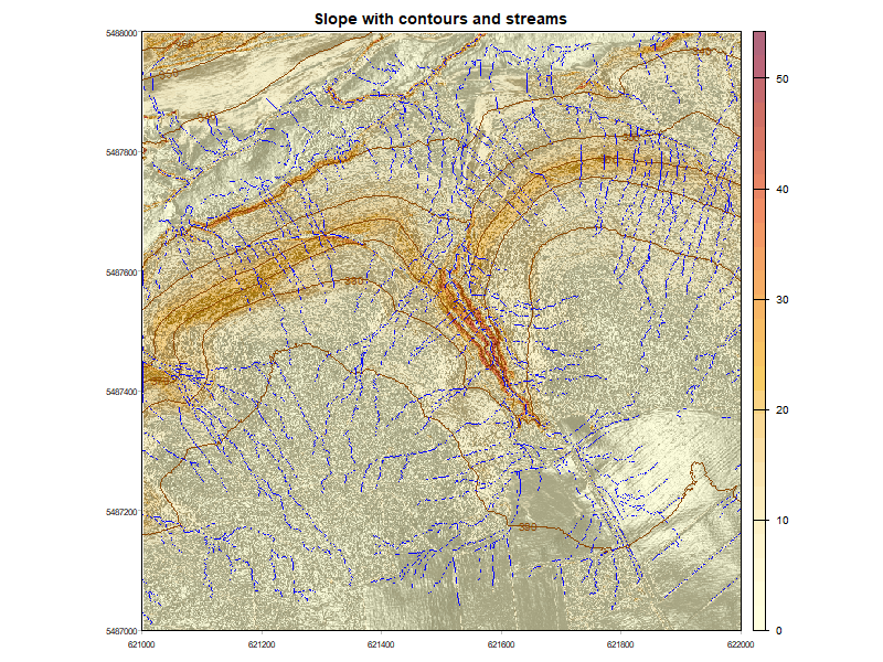
Flow accumulation comparison
plot_flow_acc(dtm, metrics = metrics)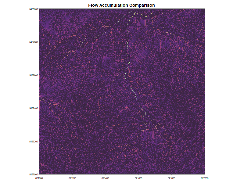
Note: In the package this is fully interactive — toggle layers and adjust opacity via a Shiny app.
Combined valleys and ridges
plot_main_networks(dtm, main_valleys = main_valleys, main_ridges = main_ridges, metrics = metrics)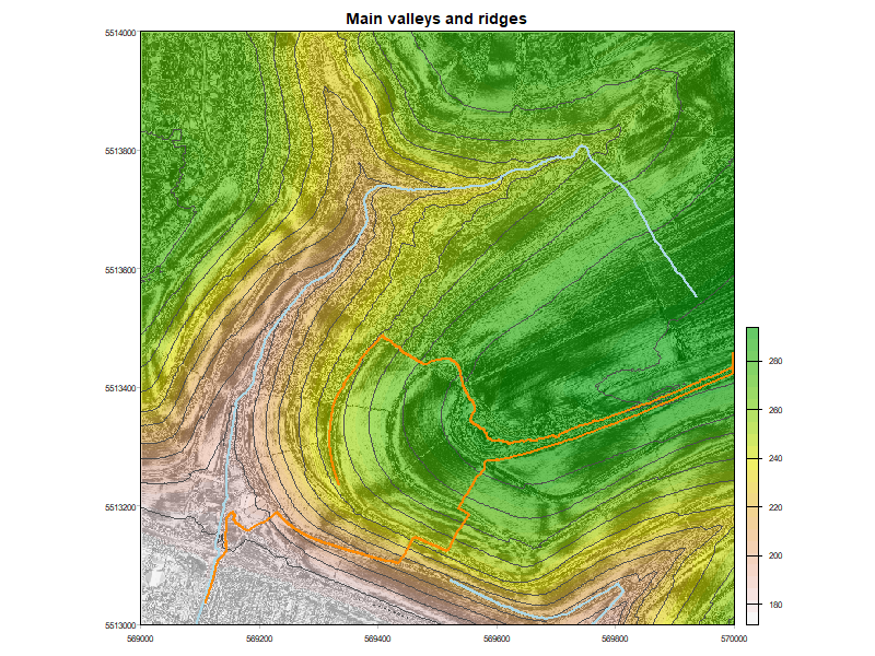
Keylines with slope and contours
plot_keylines(dtm, metrics = metrics, keylines = valley_keylines)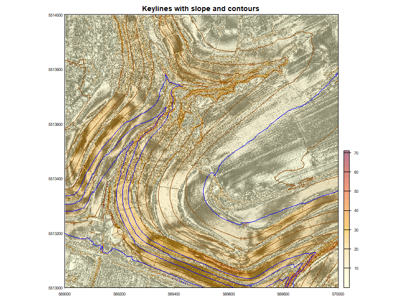
Function Reference
| Function | Description |
|---|---|
calc_geomorph_metrics() |
Calculate all terrain and hydrological metrics from a DTM |
extract_networks() |
Extract valley or ridge networks |
extract_main_valleys() |
Identify main valley lines by flow accumulation |
extract_main_ridges() |
Identify main ridge lines by flow accumulation |
create_keylines() |
Generate approximate keylines from valley or ridge lines |
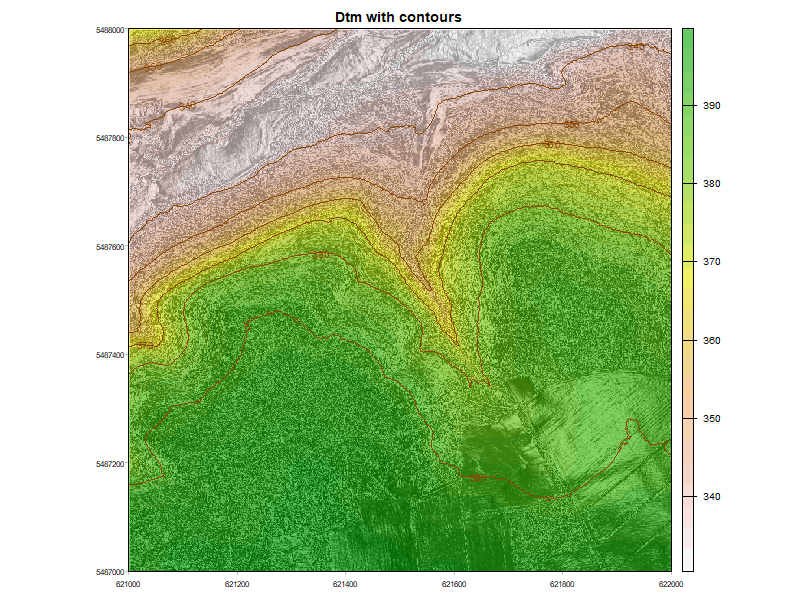
plot_dtm_contours() |
Plot DTM with hillshade and contours |
plot_slope_channels() |
Plot slope with contours and stream network |
plot_flow_acc() |
Interactive Shiny app for flow accumulation comparison |
plot_main_networks() |
Plot DTM with main valley and ridge lines |
plot_keylines() |
Plot keylines with slope and contours |
About Keyline Design
Keyline design is a land and water management methodology developed by P.A. Yeomans. It uses the natural topography of a landscape — particularly valley and ridge lines — to guide water flow and distribution across a property. This package provides computational tools to support the desktop planning phase of keyline analysis.
Acknowledgements
The algorithms in this package are based on the TopoDrain plugin, which provided the methodological foundation for the terrain analysis.